Didactical Considerations - Growth Sequences
Growth is a fruitful topic in mathematics classrooms, for mathematics concept formation and for rich application problems. Growth processes can be found in various fields of real life like biology, physics or finance. With sequences being a fundamental part of mathematics, growth sequences can be discussed at any grade at school on different difficulty levels. Linear, polynomial or exponential are the quite common examples, but also logistic growth, the most common case in reality, can be dealt with. Furthermore, there are numerous ways of representing growth sequences, like (discrete) graphs, value tables and explicit or recursive equations, making them a good possibility to convey mathematical representation competencies.
These multiple ways of representing make the use of ICT particularly fertile, because you can dynamically link representations to show connections and to make them interactively variable. There are several programs that offer ways to represent growth sequences, i.e. educational mathematics programs like Geogebra, handheld devices or spreadsheet software. A notable advantage of spreadsheet software are the way the discrete software cells are closely related to the terms of a sequence and the relative facility of creating value tables using recursive formula, which then can be represented in graphs or diagrams.  TT link
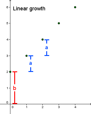
Linear growth
When describing the growth process from one step to another (a step may be a day, a month or a year) recursively defined sequence are a good mathematical model. If the difference between two immediately consecutive terms of the sequence is constant, we speak of linear growth.
When describing the growth process from one step to another (a step may be a day, a month or a year) recursively defined sequence are a good mathematical model. If the difference between two immediately consecutive terms of the sequence is constant, we speak of linear growth.
Generally:
| Equation | Table | Graph | |||||||||||||||||||||
|
f(n+1) = a + f(n) with f(0) = b or f(n) = a \cdot n + b |
|
|
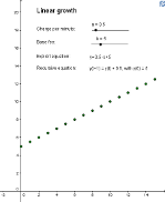
Example:
A mobile phone service provider charges 10 cents per minute with a fixed base fee of 5 € per month. With t being the number of minutes somebody telephoned in a certain month, one can visualize the costs c(t) with a (recursive or explicit) equation, a value table or a graph of a linear growth sequence:
A mobile phone service provider charges 10 cents per minute with a fixed base fee of 5 € per month. With t being the number of minutes somebody telephoned in a certain month, one can visualize the costs c(t) with a (recursive or explicit) equation, a value table or a graph of a linear growth sequence:
| Equation | Table | Graph | |||||||||||||||||||||
|
c(t+1) = 0.1 + c(t) with c(0) = 5 or c(t) = 0.1 \cdot t + 5 |
|
|
Exponential growth
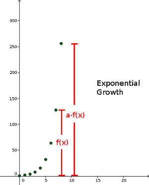
If the quotient of immediate consecutive terms is constant, we speak of exponential growth. In other words: Multiplying the immediate preceding term with a fixed constant yields in a term of the sequence. This holds true for the entire sequence.
If the quotient of immediate consecutive terms is constant, we speak of exponential growth. In other words: Multiplying the immediate preceding term with a fixed constant yields in a term of the sequence. This holds true for the entire sequence.
Generally:
| Equation | Table | Graph | |||||||||||||||||||||
|
f(n+1) = a \cdot f(n) with f(0) = 1 or f(n) = a^n |
|
|
Example:
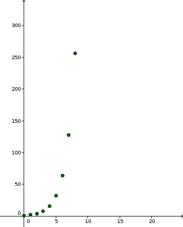
With a given sufficient space and nutrition, bacteria colonies double their number through binary fission in each step of reproduction. With b(t) being the number of bacteria after t steps and starting with one bacterium, the represent growth sequence can be represented as follows:
With a given sufficient space and nutrition, bacteria colonies double their number through binary fission in each step of reproduction. With b(t) being the number of bacteria after t steps and starting with one bacterium, the represent growth sequence can be represented as follows:
| Equation | Table | Graph | |||||||||||||||||||||
|
b(t+1) = 2 \cdot b(t) with b(0) = 1 or b(t) = 2^t |
|
|
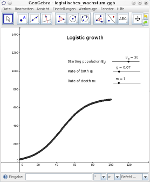
Logistic growth
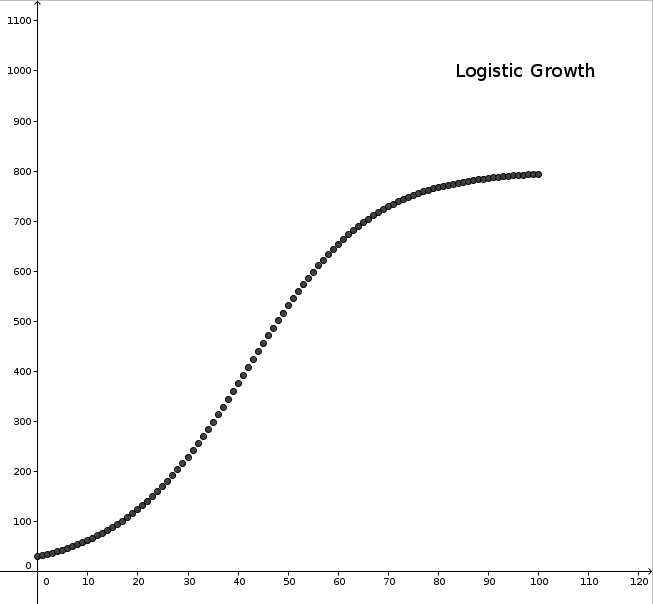
Logistic growth is a realistic model for population growth that can be used for any kind of population whose growtwh possibilities are limited. It is - in the beginning - similar to exponential growth, but with the realistic assumption of a constrained maximum population size.
The logistic growth is defined by a sequence's increase or decrease \Delta f(x) which is proportional to
or \Delta f(x) = k \cdot f(x) \cdot (G-f(x)),
with a constant k. This results in the equation below:
The logistic growth is defined by a sequence's increase or decrease \Delta f(x) which is proportional to
- the current population size f(x)
- the difference of the maximal and the current population size (G-f(x))
- the rates of reproduction and starvation of the population, which is combined in the constant k
f(x+1) = f(x) + \Delta f(x)
with \Delta f(x) \sim f(x) \cdot (G-f(x))or \Delta f(x) = k \cdot f(x) \cdot (G-f(x)),
with a constant k. This results in the equation below:
| Equation | Graph |
|
f(x+1) = f(x) + k \cdot f(x) \cdot (G-f(x)),
with f(0) = f_0 where k is the combined rate of reproduction and starvation, f_0 the initial population and G the maximal population size. There is also an explicit form of the equation: f(x) = G \cdot \left(1 + e^{-k \cdot G \cdot x} \cdot \left( \frac{G}{f_0} - 1\right)\right)^{-1} To explain this equation, we have to refer to the literature. |
|